Complex Mapping and Vibration

Overview

Visualizing complex functions is inherently challenging: the complex plane is already two-dimensional, so a function $f: \mathbb{C} \to \mathbb{C}$ requires four dimensions for a complete Cartesian graph. To overcome this, colour-coded points in 2D space represent different complex numbers, and a transformation is animated as points smoothly interpolating from the domain to the image of the function.

This project explores various complex transformations — including powers, reciprocals, and combinations — and their geometric effects on grids and scattered point clouds. Two coordinate systems are used: Cartesian grids (colour based on the real coordinate) and Polar grids (colour based on magnitude), each rendered as either discrete dots or continuous lines.

Controls: left click to trigger the animation, scroll to zoom, and middle button to pan the viewport.

Mathematical Background

Complex Transformations

A complex transformation is a function $f: \mathbb{C} \to \mathbb{C}$ that maps each point $z = x + iy$ in the domain to a new point $w = f(z)$ in the image. The geometric effect — rotation, scaling, inversion, or distortion — depends on the algebraic form of $f$ .

The functions implemented in this project include:

\begin{aligned} f(z) &= z^n \quad \text{(power, e.g. } z^2,\, z^{5.35}\text{)} \\ f(z) &= \frac{1}{z} \quad \text{(reciprocal / inversion)} \\ f(z) &= iz \quad \text{(90° rotation)} \\ f(z) &= (z+1)^{-2} \quad \text{(shifted reciprocal squared)} \\ f(z) &= \frac{1}{z^2} + 5z \quad \text{(combination)} \\ f(z) &= 3z^3 \quad \text{(scaled cubic)} \end{aligned}

Each function produces a distinct geometric signature: the power map $z^n$ multiplies the argument by $n$ and raises the modulus to the $n$ -th power, while the reciprocal $1/z$ performs a circle inversion combined with a conjugation.

Visualization Methods

Four visualization modes are available, combining two coordinate systems with two rendering styles. Each mode colours points differently: Cartesian modes map the $x$ -coordinate to a colour gradient, while Polar modes map the magnitude $|z|$ to colour. The animation interpolates each point from its original position to its transformed position under $f(z)$ .

Cartesian Dots

Thousands of randomly scattered dots fill the complex plane, each coloured by its real coordinate. When the transformation is applied, the cloud of dots flows to new positions, revealing how the function stretches, compresses, and rotates different regions of the plane.

Cartesian Lines

A regular Cartesian grid of horizontal and vertical lines is drawn, with colour varying along the $x$ -axis. Under the transformation, straight lines warp into curves, making it easy to identify conformal properties — angles between grid lines are preserved by analytic functions.

Polar Dots

Dots are distributed across the plane and coloured by their magnitude $|z|$ . This highlights how the transformation affects distance from the origin — inversions swap near and far points, while power maps expand or compress radial distances non-linearly.

Polar Lines

Concentric circles and radial rays form the polar grid, with colour encoding magnitude. The transformation bends circles into new curves and redirects rays, visually demonstrating how $f(z)$ distorts the polar structure of the plane. Unit circle is shown in white color for reference.

Transformations Gallery

The images below compare the transformation results of different complex mappings in both dots and lines rendering styles. Showing the original domain states is omitted here as they are identical to the grids shown at the top of the page.

Cartesian Dots — Reciprocal Mapping

A scattered cloud of Cartesian dots transformed by the reciprocal mapping $f(z) = 1/z$ . The dots cluster near the origin as outer points are pulled inward, revealing the inverse mapping behavior.

Cartesian Lines — Reciprocal Mapping

A regular Cartesian grid transformed by the reciprocal mapping $f(z) = 1/z$ . Straight lines are warped into circles passing through the origin, illustrating how grid structures deform.

Cartesian Dots — Power Mapping

Applying a power function such as $f(z) = \frac{1}{(z+1)^2}$ to scattered Cartesian dots. The squaring map doubles angles and squares magnitudes, causing the dot cloud to wrap around the origin.

Cartesian Lines — Combination Function

A more exotic transformation such as $f(z) = 1/z^2 + 5z$ applied to the Cartesian grid. The interplay between singular and linear terms creates intricate swirling patterns.

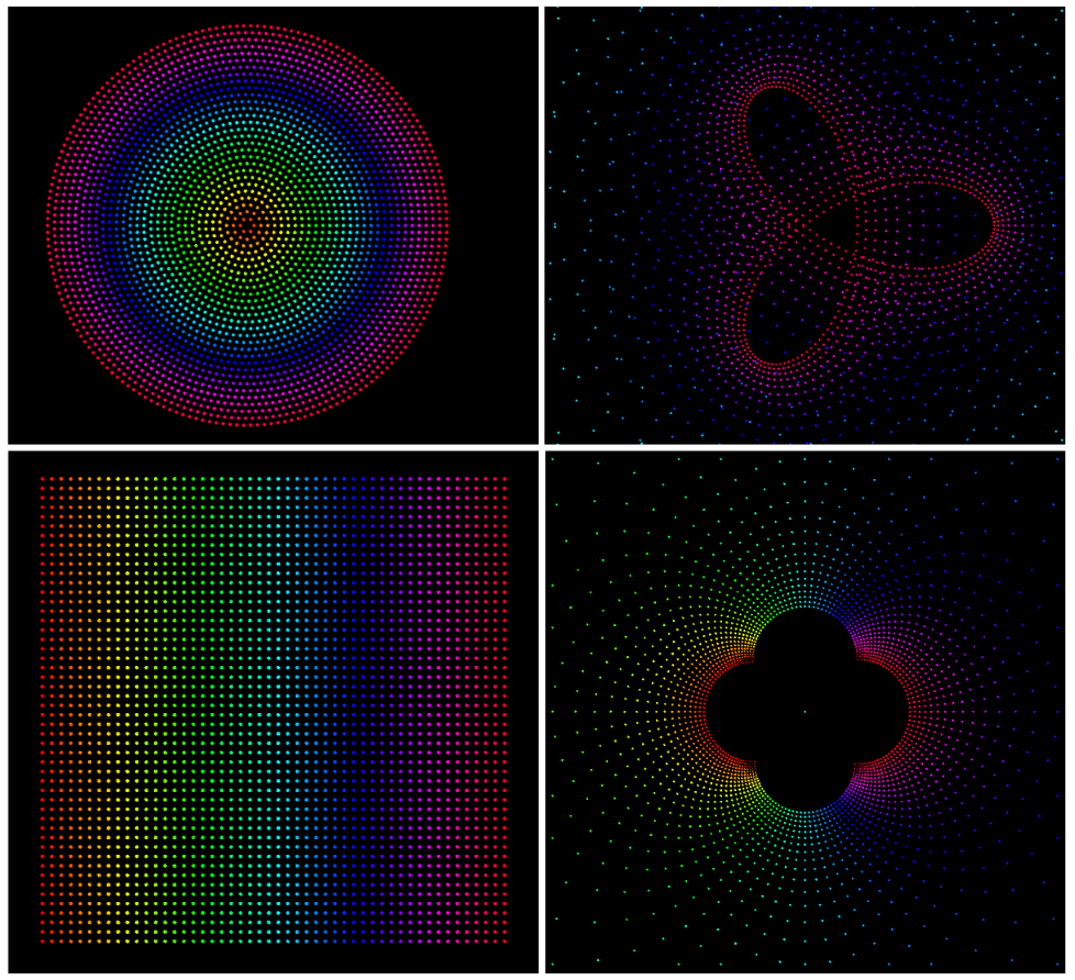
Polar Dots — Reciprocal Power

The result of a polar dots reciprocal power mapping accodring to $f(z) = \frac{1}{z^3+1}$ . Formerly outer (far) dots now cluster near the origin and vice versa, visually inverting the magnitude-based radial color gradient.

Polar Lines — Power Mapping

The result of a polar grid lines power mapping. The circles and radial rays are warped into new curve families, demonstrating how $f(z) = z^3$ triples the angular spacing and cubes the distances.

Additional Examples

The following videos showcase various complex transformations animated in real time. Click on any video to open it in full resolution and view the dynamic mapping behavior.

Polar Dots — Inversion

f(z) = \frac{1}{z^3+1}

This is one of the most beautiful transformations I have come acrosss. The dots rotate themselves around 3 specific points, probably related to the geometry of the complex plane, and how this function affects it.

Cartesian Dots — Reciprocal

f(z) = 1/z

Dots mapped by inversion, showing points flowing across the unit circle boundary.

Cartesian Lines — Reciprocal

f(z) = 1/z

Lines warping into nested, orthogonal circular arcs intersecting at the origin.

Polar Lines — Cubic

f(z) = z^3

Grid mapping that wraps the plane three times, compressing the interior.

Cartesian Dots — Power

f(z) = z^{5.35}

Fractional exponent creating overlapping sheets and spiral dislocation.

Cartesian Dots — Shifted Pole

f(z) = (z+1)^{-2}

Singularity at z = -1 pulling grid structure into a dramatic outward flow.

Cartesian Dots — Scaled Cubic

f(z) = 3z^3

Cubic expansion mapping showing three-fold symmetric warp of the dot cloud.

Technology Stack

This project was built using Processing (Java-based creative coding framework), leveraging its real-time rendering pipeline for smooth animations of thousands of points. A custom Complex class implements arithmetic operations (addition, subtraction, multiplication, power, reciprocal, polar conversion) used to evaluate transformations at each point.

ProcessingJavaComplex AnalysisReal-time RenderingInteractive VisualizationColor Mapping

Source Code

Cartesian Mapping (Dots) Repository Cartesian Mapping (Lines) Repository